I came across the Iris dataset on Github, inquisitive about the topic I decided to work on this dataset while trying to put it across in a simpler way for everyone to understand.

Dataset link : bit.ly/2R6ZXqB

Source : Sebastian Raschka (rasbt)

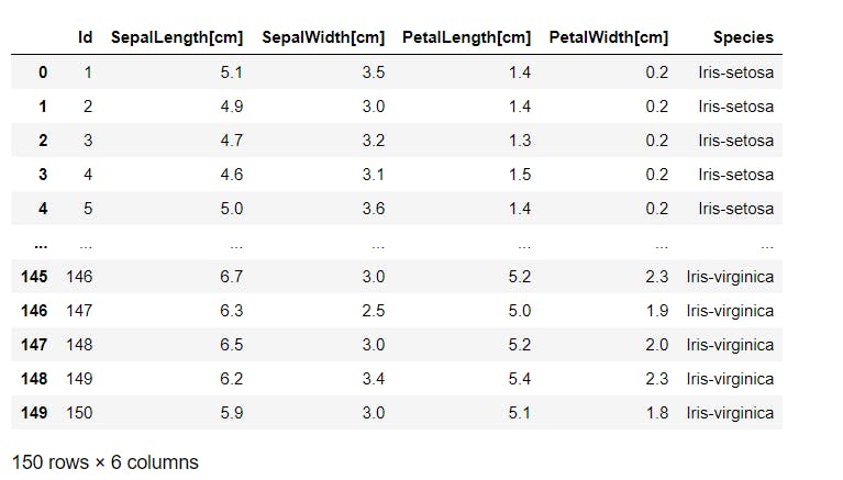
The dataset consists of various features like SepalLength[cm], SepalWidth[cm], PetalLength[cm], PetalWidth[cm] which can help us to determine that the input data belongs to which species. The Iris dataset comprises various species like Iris-setosa, Iris-versicolor, Iris-virginica.

Here, I have tried to analyze the data and then implemented a machine learning model to classify new data based on their input features.

Libraries :

Pandas - provides several methods for reading data in different formats.

Matplotlib and seaborn - used for plotting basic and advanced visualizations respectively.

#Import libraries
import pandas as pd
import matplotlib.pyplot as plt
import seaborn as sns

Reading and Displaying data :

#load the dataset
iris = pd.read_csv("iris.csv")

#Reading and displaying the dataset
iris

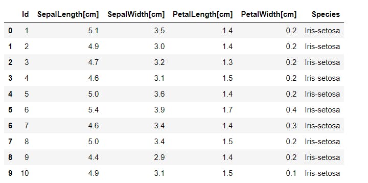
# Display only top rows (By default 5)
iris.head(10)

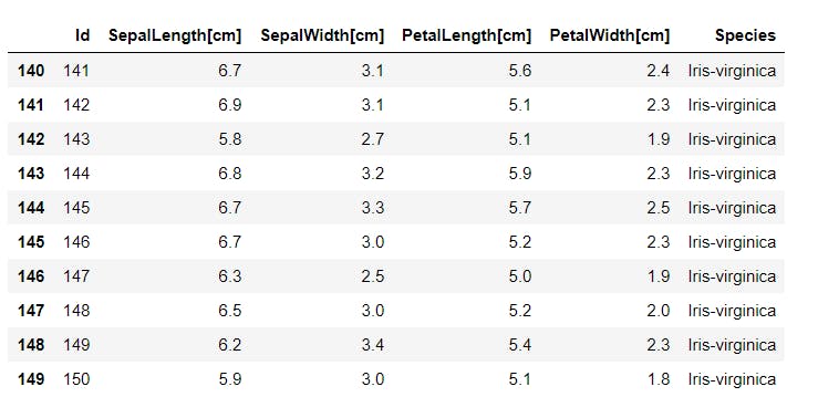
# Display only bottom rows (By default 5)
iris.tail(10)

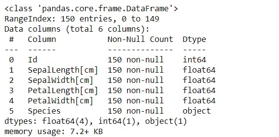
Information about dataframe :

The information tells us about the number of non-missing values and the data type of each column in the dataframe.

#To get information about the dataframe.
iris.info()

Alternate way to check the number of missing values and data type of each column -

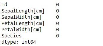
#To check for missing values
iris.isnull().sum()

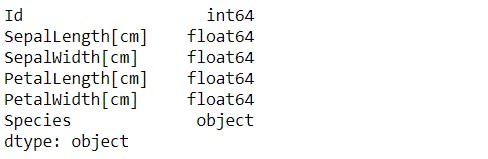
#To check the datatype of your dataframe
iris.dtypes

To check the unique values in the "Species" column -

#Check the class labels
iris["Species"].unique()

Convert the "Species" column into numeric format :

Machine learning algorithms can then decide in a better way how those labels must be operated. It is an important pre-processing step for the structured dataset in supervised learning.

#Now convert the Species column into numeric format
dict1 = {'Iris-setosa' : 0, 'Iris-versicolor' : 1, 'Iris-virginica' : 2}
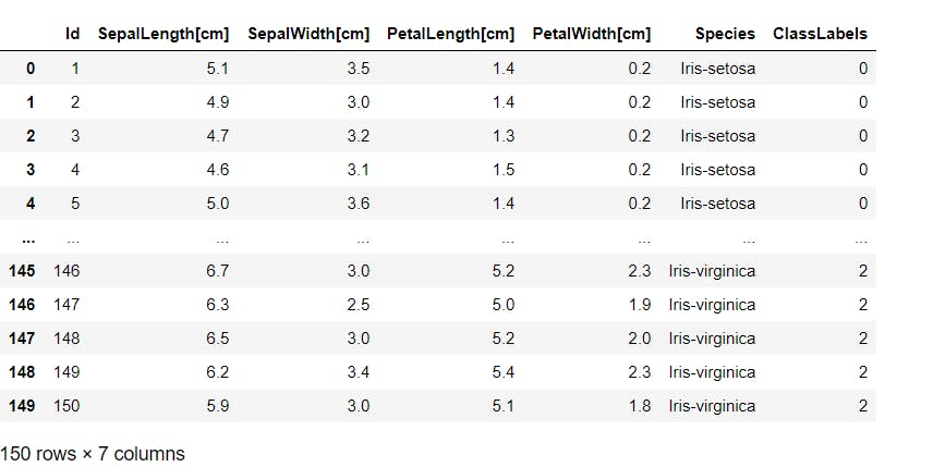
iris["ClassLabels"] = iris["Species"].map(dict1)

#Displaying the dataset
iris

Shuffling the dataset :

As we can see that the dataset was organized based on the species column, we need to shuffle it so that there is no bias observed while training the model and also we can train the model where it covers training data of species of all types for better accuracy.

#Copy of Original dataframe
iris_copy = iris.copy()

#Shuffling the dataframe
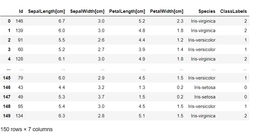
iris_shuffled = iris_copy.sample(frac=1).reset_index(drop=True)
iris_shuffled

Visualization :

The pair plot visualization helps to plot the graph of all the input features with each other as well as the output label.

This helps to understand the correlation between each feature in the dataset.

#Pair plot
sns.pairplot(data=iris_shuffled, hue ="ClassLabels")
plt.show()

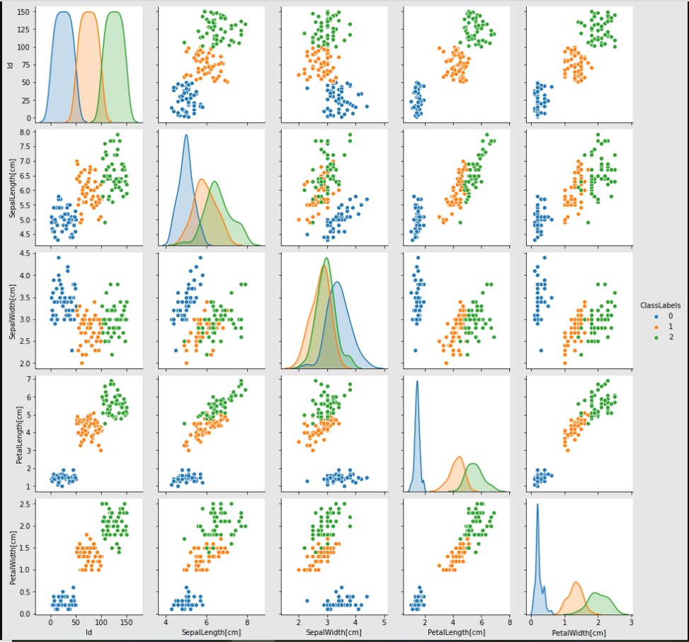We can see that the input features - PetalLength[cm] and PetalWidth[cm] are highly correlated and the different data points of different species do not overlap with each other.

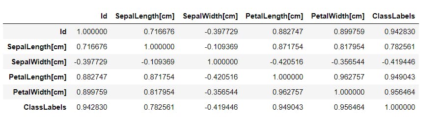
To see the correlation between the features in the numerical form between 0 and 1, we use the below code. The higher the value, the stronger is the correlation between the features.

#To find the correlation between the input feature and the output label
iris_shuffled.corr()

Machine Learning :

Input Features and Output Label :

# Input features (X) and Output label (y)
X = iris_shuffled[["PetalLength[cm]", "PetalWidth[cm]"]]
y = iris_shuffled["ClassLabels"]

Splitting the data :

We split the dataset into training and test set. The machine learning model is trained on the training set and the testing set is used to determine the accuracy of the model to predict output on the unseen dataset.

# Import train_test_split
from sklearn.model_selection import train_test_split

# Splitting of data
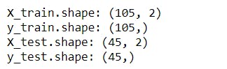
X_train, X_test, y_train, y_test = train_test_split(X,y, test_size=0.3, random_state = 123, shuffle = True)

The above code splits the dataset into 30% as a test set and the remaining 70% as the training set.

print(f'X_train.shape: {X_train.shape}')
print(f'y_train.shape: {y_train.shape}')
print(f'X_test.shape: {X_test.shape}')
print(f'y_test.shape: {y_test.shape}')

Supervised Learning -

The dataset consists of the labelled data, therefore it is a supervised machine learning project.

This is a Classification problem, as we need to classify the input features.

K - Nearest Neighbors :

K-NN algorithm assumes the similarity between the new case/data and available cases and puts the new case into the category that is most similar to the available categories.

Fitting the model :

# Fit k - nearest neighbors
from sklearn.neighbors import KNeighborsClassifier

knn_model = KNeighborsClassifier(n_neighbors=3)
knn_model.fit(X_train, y_train)

Prediction : To predict the output of testing data.

# To make predictions on test data.
y_pred = knn_model.predict(X_test)
y_pred

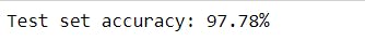
Accuracy : To check the accuracy of the output of the machine learning model on test dataset.

# To check the accuracy of the model.
accuracy = knn_model.score(X_test,y_test) * 100
print(f'Test set accuracy: {accuracy:.2f}%')

Yay! 🥳 You made it till the end. Hope you found it interesting.